Constraint Generation in the Presence of Bad Data
Posted on Thu 21 September 2017 in TDDA
Bad data is widespread and pervasive.1
Only datasets and analytical processes that have been subject to rigorous and sustained quality assurance processes are typically capable of achieving low or zero error rates. "Badness" can take many forms and have various aspects, including incorrect values, missing values, duplicated entries, misencoded values, values that are inconsistent with other entries in the same dataset, and values that are inconsistent with those in other datasets, to name but a few.
We have previously discussed automatic constraint discovery and verification as a mechanism for finding, specifying, and executing checks on data, and have advocated using these to verify input, output, and intermediate datasets. Until now, however, such constraint discovery has been based on the assumption that the datasets provided to the discovery algorithm contain only good data—a significant limitation.
We have recently been thinking about ways to extend our approach to constraint generation to handle cases in which this assumption is relaxed, so that the "discovery" process can be applied to datasets that include bad data. This article discusses and illustrates one such approach, which we have prototyped, as usual, in our own Miró software. We plan to bring the same approach to the open-source Python tdda library as soon as we have gained further experience using it and convinced ourselves we are going in a good direction.
The most obvious benefit of extending constraint generation to function usefully even when the dataset used contains some bad data is increased applicability. Perhaps a more important benefit is that it means that, in general, more and tighter constraints will be generated, potentially increasing their utility and more clearly highlighting areas that should be of concern.
The Goal and Pitfalls: "Seeing Through" Bad Data
Our aim is to add to constraint generation a second mode of operation whose goal is not to discover constraints that are true over our example data, but rather to generate constraints for which there is reasonable evidence, even if some of them are not actually satisfied by all of the example data. This is not so much constraint discovery as constraint suggestion. We want the software to attempt to "see through" the bad data to find constraints similar to those that would have been discovered had there been only good data. This is hard (and ill specified) because the bad data values are not identified, but we shall not be deterred.
For constraints generated in this way, the role of a human supervisor is particularly important: ideally, the user would look at the constraints produced—both the ordinary ones actually satisfied by the data and the more numerous, tighter suggestions typically produced by the "assuming bad data" version—and decide which to accept on a case-by-case basis.
Extending constraint generation with the ability to "see through" bad data is very powerful, but carries obvious risks: as an example, constraint suggestion might look at lending data and conclude that defaults (non-payment of loans—hopefully a small proportion of customers) are probably outliers that should be excluded from the data. Clearly, that would be the wrong conclusion.
Notwithstanding the risks, our initial experiences with generation in the presence of bad data have been rather positive: the process has generated constraints that have identified problems of which we had been blissfully unaware. The very first time we used it highlighted:
- a nearly but not-quite unique identifier (that should, of course, have been unique)
- a number of low-frequency, bad categorical values in a field
- several numeric fields with much smaller true good ranges than we had realized.
Additionally, even when the constraints discovered go beyond identifying incorrect data, they often highlight data that we are happy to have flagged because they do represent outliers deserving of scrutiny.
Our Approach
Our initial attempt at extending constraint discovery to the case in which there is (or might be) bad data is straightforward: we simply allow that a proportion of the data might be bad, and look for the best constraints we can find on that basis.
With our current implementation, in Miró, the user has to supply an upper limit on the proportion, p, of values that are thought likely to be bad. Eventually, we expect to be able to determine this proportion heuristically, at least by default. In practice, for datasets of any reasonable size, we are mostly just using 1%, which seems to be working fairly well.
We should emphasize that the "bad" proportion p provided is not an estimate of how much of the data is bad, but an upper limit on how much we believe is reasonably likely to be bad.2 As a result, when we use 1%, our goal is not to find the tighest possible constraints that are consistent with 99% of data, but rather to work with the assumption that at least 99% of the data values are good, and then to find constraints that separate out values that look very different from the 99%. If this turns out to be only 0.1%, or 0.001%, or none at all, so much the better.
The way this plays out is different for different kinds of constraint. Let's work through some examples.
Minimum and Maximum Constraints
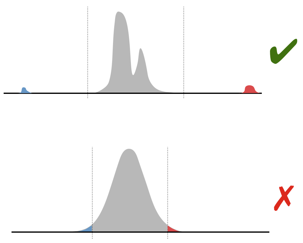
Looking for minimum and maximum constraints in the presence of possible bad values is closely connected to univariate outlier detection. We cannot, however, sensibly make any assumptions about the shape of the data in the general case, so parametric statistics (means, variances etc.) are not really appropriate. We also need to be clear that what we are looking for is not the tails of some smooth distribution, but rather values that look as if they might have been generated by some completely different process, or drawn from some other distribution.
An example of the kind of thing what we are looking for is something qualitatively like the situation in the top diagram (though perhaps considerably more extreme), where the red and blue sections of the distribution look completely different from the main body, and we want to find cutoffs somewhere around the values shown. This is the sort of thing we might see, for example, if the main body of values are prices in one currency and the outliers, in contrast, are the similar prices, but measured in two other currencies. In contrast, we are not aiming to cut off the tails of a smooth, regular distribution, such as the normal distribution shown in the lower diagram.
In our initial implementation we have used the possible bad proportion p to define an assumed "main body" of the distribution as running between the quantiles at (1 – p) and p (from the 1st percentile to the 99th, when p = 1%). We assume all values in this range are good. We then search out from this main body of the distribution, looking for a gap between successive values that is at least α times the (1% – 99%) interquantile range. We are using α=0.5 for now. Once we have identified a gap, we then pick a value within it, currently favouring the end nearer the main distribution and also favouring "round" numbers.
Let's look at an example.
We have a dataset with 12,680,141 records and 3 prices (floating-point values), Price1, Price2 and Price3, in sterling. If we run ordinary TDDA constraint discovery on this, we get the following results:
| Individual Field Constraints | |||||||
|---|---|---|---|---|---|---|---|
| Name | Type Allowed | Min Allowed | Max Allowed | ||||
| Price1 | real | 0.0 | 198,204.34 | ||||
| Price2 | real | –468,550,685.56 | 2,432,595.87 | ||||
| Price3 | real | 0.0 | 1,390,276,267.42 | ||||
With ordinary constraint discovery, the min and max constraints are just set to the largest and smallest values in the dataset, so this tells us that the largest value for Price1 in the dataset is nearly £200,000, that Price2 ranges from close to –£500m to about +£2.5m, and that Price3 runs up to about £1.4bn.
If we rerun the constraint generation allowing for up to 1% bad data, we get the following instead.
| Individual Field Constraints | |||||||
|---|---|---|---|---|---|---|---|
| Name | Type Allowed | Min Allowed | Max Allowed | ||||
| Price1 | real | 0.0 | 38,000.0 | ||||
| Price2 | real | –3,680.0 | 3,870.0 | ||||
| Price3 | real | 0.0 | 125,000.0 | ||||
Let's look at why these values were chosen, and see whether they are reasonable.
Starting with Price1, let's get a few more statistics.
| min Price1 | percentile 1 Price1 | median Price1 | percentile 99 Price1 | max Price1 |
|---|---|---|---|---|
| 0.00 | 24.77 | 299.77 | 2,856.04 | 198,204.34 |
So here our median value is just under £300, while our first percentile value is about £25 and our 99th percentile is a little under £3,000, giving us an interquantile range also somewhat under £3,000 (£2,831.27, to be precise).
The way our algorithm currently works, this interquantile range defines the scale for the gap we need to define something as an outlier—in this case, half of £2,831.27, which is about £1,415.
If we were just looking to find the tighest maximum constraint consistent with 1% of the data being bad (with respect to this constraint), we would obviously just set the upper limit to fractionally above £2,856.04. But this would be fairly nonsensensical as we can see if we look at the data around that threshold. It is a feature of this particular data that most values are duplicated a few times (typically between 3 and 10 times), so we first deduplicate them. Here are the first 20 distinct values above £2,855:
2,855.02   2,855.42   2,855.80   2,856.04
2,855.16   2,855.50   2,855.82   2,856.08
2,855.22   2,855.64*  2,855.86   2,856.13
2,855.38   2,855.76   2,855.91   2,856.14
Obviously, there's nothing special about £2,854.04 (marked with *), and there is no meaningful gap after it, so that would be a fairly odd place to cut off.
Now let's look at the (distinct) values above £30,000:
30,173.70   31,513.21   39,505.67   44,852.01   67,097.01    72,082.60
30,452.45   32,358.52   39,703.93   45,944.21   60,858.88    72,382.57
30,562.55   32,838.23   40,888.79   47,026.70   60,911.84    72,388.55
30,586.96   33,906.98   40,999.04   47,058.99   63,160.28    72,657.04
30,601.67   34,058.27   41,252.50   47,126.60   63,984.64    72,760.90
30,620.78   35,302.33   41,447.00   49,827.28   64,517.16    90,713.28
31,118.10   36,472.53   41,513.95   51,814.22   67,256.27   103,231.44
31,139.86   36,601.86   42,473.36   53,845.76   68,081.68   123,629.97
31,206.71   36,941.76*  43,384.46   55,871.84   70,782.28   198,204.34
31,449.57   39,034.38   43,510.03   56,393.14   71,285.95
The cutoff the TDDA algorithm has chosen (£38,000) is just after the value marked *, which is the start of the first sizable gap. We are not claiming that there is anything uniquely right or "optimal" about the cutoff that has been chosen in the context of this data, but it looks reasonable. The first few values here are still comparatively close together—with gaps of only a few hundred between each pair of successive value—and the last ones are almost an order of magnitude bigger.
We won't look in detail at Price2 and Price3, where the algorithm has narrowed the range rather more, except to comment briefly on the negative values for Price2, which you might have expected to be excluded. This table shows why:3
| countnegative Price2 | countzero Price2 | countpositive Price2 | countnull Price2 | countnonnull Price2 |
|---|---|---|---|---|
| 1,300 | 51,640 | 39,750 | 15,880 | 92,690 |
Although negative prices are not very common, they do account for about 1.2% of the data (critically, more than 1%). Additionally, nearly 15% of the values for Price2 are missing, and we exclude nulls from this calculation, so the truly relevant figure is that 1,300 of 92,690 non-null values are negative, or about 1.4%.
Other Constraints
We will now use a slightly wider dataset, with more field types, to look at how constraint generation works for other kinds of constraints in the presence of bad data. Here are the first 10 records from a dataset with 108,559 records, including a similar set of three price fields (with apologies for the slightly unintuitive colouring of the Colour field).
| ID | Date | Price1 | Price2 | Price3 | Code | nItems | Parts | Colour |
|---|---|---|---|---|---|---|---|---|
| af0370b4-16e4-1891-8b30-cbb075438394 | 2016-11-01 00:38:34 | 830.25 | ∅ | 830.25 | NLOM | 1 | 62444 | red |
| 126edf08-16e5-1891-851c-d926416373f2 | 2016-11-01 00:41:21 | 983.08 | 0.00 | 983.08 | QLDZ | 1 | 62677 | yellow |
| 73462586-16ed-1891-b164-7da16012a3ab | 2016-11-01 01:41:20 | 540.82 | 0.00 | 540.82 | TKNX | 1 | 62177 62132 | red |
| 1cd55aac-170e-1891-aec3-0ffc0ab020e7 | 2016-11-01 05:35:08 | 398.89 | 0.00 | 398.89 | PKWI | 1 | 61734 | red |
| 68f74486-170e-1891-8b30-cbb075438394 | 2016-11-01 05:37:16 | 314.54 | 8.21 | 314.54 | PLUA | 1 | 62611 | red |
| 28dff654-16fa-1891-bd69-03d25ee96dee | 2016-11-01 03:12:18 | 479.75 | ∅ | 479.75 | UHEG | 1 | 62128 | red |
| 14321670-1703-1891-ab75-77d18aced2f5 | 2016-11-01 04:16:09 | 733.41 | 0.00 | 733.41 | RTKT | 2 | 61829 | red |
| 60957d68-1717-1891-a5b2-67fe1e248d60 | 2016-11-01 06:41:27 | 537.81 | 0.00 | 537.81 | OBFZ | 1 | 61939 62371 | red |
| 4fea2bb6-171d-1891-80a6-2f322b85f525 | 2016-11-01 07:23:56 | 132.60 | 2.42 | 135.02 | TACG | 2 | 62356 | red |
| 204ed3d6-1725-1891-a1fb-15b6ffac52ce | 2016-11-01 08:19:52 | 866.32 | ∅ | 866.32 | XHLE | 2 | 61939 | red |
If we run ordinary constraint discovery on this (not allowing for any bad data), these are the results:
| Individual Field Constraints | ||||||||
|---|---|---|---|---|---|---|---|---|
| Name | Type Allowed | Min Allowed | Max Allowed | Sign Allowed | Nulls Allowed | Duplicates Allowed | Values Allowed | # Regular Expressions |
| ID | string | length 32 | length 36 | 0 | - | 2 | ||
| Date | date | 1970-01-01 | 2017-06-03 23:59:06 | 0 | ||||
| Date:time-before-now | timedelta | 107 days, 11:28:05 | 17428 days, 11:27:11 | positive | ||||
| Price1 | real | 0.0 | 19,653,405.06 | non-negative | 0 | |||
| Price2 | real | -4,331,261.54 | 589,023.50 | |||||
| Price3 | real | 0.0 | 20,242,428.57 | non-negative | 0 | |||
| Code | string | length 4 | length 4 | 0 | - | 3 | ||
| nItems | int | 1 | 99 | positive | - | |||
| Parts | string | length 5 | length 65 | 1 | - | 5 | ||
| Colour | string | length 3 | length 6 | 0 | - | 6 values | 2 | |
There are a few points to note:
- To make the table more manageable, the regular expressions and field values are not shown, by default. We'll see them later.
- The third line of constraints is generated is slightly different from the others, and looks not at the actual values of the dates, but rather than how far in the past or future they are. This is something else we are experimenting with, but doesn't matter too much for this example.
Let's repeat the process telling the software that up to 1% of the data might be bad.
| Individual Field Constraints | ||||||||
|---|---|---|---|---|---|---|---|---|
| Name | Type Allowed | Min Allowed | Max Allowed | Sign Allowed | Nulls Allowed | Duplicates Allowed | Values Allowed | # Regular Expressions |
| ID | string | length 32 | length 36 | 0 | no | 1 | ||
| Date | date | 1970-01-01 01:23:20 | 2017-06-03 23:59:06 | 0 | ||||
| Date:time-before-now | timedelta | 107 days, 11:55:27 | 17428 days, 11:54:33 | positive | ||||
| Price1 | real | 0.0 | 25000.0 | non-negative | 0 | |||
| Price2 | real | -520.0 | 790.0 | |||||
| Price3 | real | 0.0 | 24000.0 | non-negative | 0 | |||
| Code | string | length 4 | length 4 | 0 | - | 2 | ||
| nItems | int | 1 | 10 | positive | 0 | - | ||
| Parts | string | length 5 | length 65 | 0 | - | 2 | ||
| Colour | string | length 3 | length 6 | 0 | - | 3 values | 1 | |
Now let's consider the (other) constraint kinds in turn.
Sign
Nothing has changed for any of the sign constraints. In general, all that we do in this case is see whether less than our nominated proportion p is negative, or less than our nominated proportion p is positive, and if so write a constraint to this effect, but in the example nothing has changed.
Nulls
The nulls allowed constraint puts an upper limit on the number of nulls allowed in a field. The only two values we ever use are 0 and 1, with 0 meaning that no nulls are allowed and 1 meaning that a single null is allowed. The Parts field originally had a value of 1 here, meaning that there is a single null in this field in the data, and therefore the software wrote a constraint that a maxumim of 1 null is permitted. When the software is allowed to assume that 1% of the data might be bad, a more natural constraint is not to allow nulls at all.
No constraint on nulls was produced for the field nItems originally, but now we have one. If we check the number of nulls in nItems, it turns out to be just 37 or around 0.03%. Since that is well below our 1% limit, a "no-nulls" constraint has been generated.
Duplicates
In the original constraint discovery, no constraints banning duplicates were generated, whereas in this case ID did get a "no duplicates" constraint. If we count the number of distinct values in ID, there are in fact, 108,569 for 108,570 records, so there is clearly one duplicate, affecting 2 records. Since 2/108,570 is again well below our 1% limit (more like 0.002%), the software generates this constraint.
Values allowed.
In the original dataset, a constraint on the values for the field Colour was generated. Specifically, the six values it allowed were:
"red" "yellow" "blue" "green" "CC1734" "???"
When we ran the discovery process allowing for bad data, the result was that only 3 values were allowed, which turn out to be "red", "yellow", and "blue". If we look at the breakdown of the field, we will see why.
| Colour | count |
|---|---|
| red | 88,258 |
| yellow | 10,979 |
| blue | 8,350 |
| green | 978 |
| CC1734 | 4 |
| ??? | 1 |
The two values we might have picked out as suspicious (or at least,
having a different form from the others) are obviously CC1734 and ???,
and constraint generation did exclude those, but also green, which
we probably would not have done. There are 978 green values (about 0.9%),
which is slighty under out 1% cutoff, so it can be excluded by the
algorithm, and is. The algorithm simply works through the values in order,
starting with the least numerous one, and removes values until the maximum
possible bad proportion p is reached (cumulatively).
Values with the same frequency are treated together, which means that if
we had had another value (say "purple") with exactly the same frequency
as green (978), neither would have been excluded.
Regular Expressions
Sets of regular expressions were generated to characterize each of the four string fields, and in every case the number generated was smaller when assuming the possible presence of bad data than when not.
For the ID field, two regular expressions were generated:
^[0-9a-f]{32}$
^[0-9a-f]{8}\-[0-9a-f]{4}\-1891\-[0-9a-f]{4}\-[0-9a-f]{12}$
The first of these just corresponds to a 32-digit hex number, while the second is a 32-digit hex number broken into five groups of 8, 4, 4, 4, and 12 digits, separated by dashes—i.e. a UUID.4
If we get Rexpy to give us the coverage information We see that all but three of the IDs are properly formatted UUIDs, with just three being plain 32-digit numbers.
| Regular Expression | Incremental Coverage |
|---|---|
| ^[0-9a-f]{8}\-[0-9a-f]{4}\-1891\-[0-9a-f]{4}\-[0-9a-f]{12}$ | 108,567 |
| ^[0-9a-f]{32}$ | 3 |
and indeed, it is the 3 records that are excluded by the constraint generation assuming bad data.
We won't go through all the cases, but will look at one more. The field Parts is a list of 5-digit numbers, separated by spaces, with a single one being generated most commonly. Here are the regular expressions that Rexpy generated, together with the coverage information.
| Regular Expression | Incremental Coverage |
|---|---|
| ^\d{5}$ | 99,255 |
| ^\d{5} \d{5}$ | 8,931 |
| ^\d{5} \d{5} \d{5}$ | 378 |
| ^\d{5} \d{5} \d{5} \d{5}$ | 4 |
| ^61000 61000 61000 61000 61000 61000 61000 61000 61000 61000 61000$ | 1 |
As you can see, Rexpy has generated five separate regular expressions, where in an ideal world we might have preferred it produced a single one:
^\d{5}( \d{5})*$
In fact, however, the fact it has produced separate expressions for five clearly distinguishable cases turns out to be very helpful for TDDA purposes.
In this case, we can see that the vast bulk of the cases have either one or two 5-digit codes (which are the two regular expressions retained by constraint generation), but we would almost certainly consider the 382 cases with three and four codes to be also correct. The last one is more interesting. First, the number of codes (eleven) is noticably larger than for any other record. Secondly, the fact that it is eleven copies of a single code, that is a relatively round number is suspicious. (Looking at the data, it turns out that in no other case are any codes repeated when there are multiple codes, suggesting even more strongly that there's something not right with this record.)
Verifying the Constraint Generation Data Against the Suggested Constraints
With the previous approach to constraint discovery, in which we assume that the example data given to us contains only good data, it should always be the case that if we verify the example data against constraints generated against it, they will all pass.5 With the new approach, this is no longer the case, because our hope is that the constraints will help us to identify bad data. We show below the result of running verification against the generated contraints for the example we have been looking at:
|
|
|
|
||||||||
|
|
|
|
We can also see a little more information about where the failures were in the table below.
| Name | Failures | Type | Minimum | Maximum | Sign | Max Nulls | Duplicates | Values | Rex | |||||||||||||||||
|---|---|---|---|---|---|---|---|---|---|---|---|---|---|---|---|---|---|---|---|---|---|---|---|---|---|---|
| Values | Constraints | Allowed | Actual | ✓ | Allowed | Actual | ✓ | Allowed | Actual | ✓ | Allowed | Actual | ✓ | Allowed | Actual | ✓ | Allowed | Actual | ✓ | Allowed | Actual | ✓ | Allowed | Actual | ✓ | |
| Colour | 983 | 2 | string | string | ✓ | length 3 | length 3 | ✓ | length 6 | length 6 | ✓ | - | - | - | 0 | 0 | ✓ | - | - | - | 3 values | e.g. "green" | ✗ | 1 pattern | e.g. "???" | ✗ |
| Parts | 384 | 2 | string | string | ✓ | length 5 | length 5 | ✓ | length 65 | length 65 | ✓ | - | - | - | 0 | 1 | ✗ | - | - | - | - | - | - | 2 patterns | e.g. "62702 62132 62341" | ✗ |
| Price2 | 281 | 2 | real | real | ✓ | -520.00 | -4,331,261.54 | ✗ | 790.00 | 589,023.50 | ✗ | - | - | - | - | 15880 | - | - | - | - | - | - | - | - | - | - |
| Price3 | 92 | 1 | real | real | ✓ | 0.00 | 0.00 | ✓ | 24,000.00 | 20,242,428.57 | ✗ | ≥ 0 | ✓ | ✓ | 0 | 0 | ✓ | - | - | - | - | - | - | - | - | - |
| Price1 | 91 | 1 | real | real | ✓ | 0.00 | 0.00 | ✓ | 25,000.00 | 19,653,405.06 | ✗ | ≥ 0 | ✓ | ✓ | 0 | 0 | ✓ | - | - | - | - | - | - | - | - | - |
| nItems | 44 | 2 | int | int | ✓ | 1 | 1 | ✓ | 10 | 99 | ✗ | > 0 | ✓ | ✓ | 0 | 37 | ✗ | - | - | - | - | - | - | - | - | - |
| Code | 4 | 1 | string | string | ✓ | length 4 | length 4 | ✓ | length 4 | length 4 | ✓ | - | - | - | 0 | 0 | ✓ | - | - | - | - | - | - | 2 patterns | e.g. "A__Z" | ✗ |
| ID | 3 | 2 | string | string | ✓ | length 32 | length 32 | ✓ | length 36 | length 36 | ✓ | - | - | - | 0 | 0 | ✓ | no | e.g. "374e4f9816e51891b1647da16012a3ab" | ✗ | - | - | - | 1 pattern | e.g. "374e4f9816e51891b1647da16012a3ab" | ✗ |
| Date | 3 | 1 | date | date | ✓ | 1970-01-01 01:23:20 | 1970-01-01 | ✗ | 2017-06-03 23:59:06 | 2017-06-03 23:59:06 | ✓ | - | - | - | 0 | 0 | ✓ | - | - | - | - | - | - | - | - | - |
| Date:time-before-now | 2 | 1 | - | - | - | 109 days, 16:27:17 | 109 days, 16:28:09 | ✓ | 17430 days, 16:26:23 | 17430 days, 16:27:15 | ✗ | > 0 | ✓ | ✓ | - | 0 | - | - | - | - | - | - | - | - | - | - |
Because the verification fails in this way, and in doing so creates indicator fields for each failing constraint, and an overall field with the number of failures for each record, it is then easy to narrow down to the data being flagged by these constraints to see whether the constraints are useful or over zealous, and adjust them as necessary.
Summary
In this post, we've shown how we're extending Automatic Constraint Generation in TDDA to cover cases where the datasets used are not assumed to be perfect. We think this is quite a significant development. We'll use it a bit more, and when it's solid, extend the open-source tdda library to include this functionality.
-
As previously, I am aware that, classically, data is the plural of datum, and that purists would prefer the assertion to be "bad data are widespread and pervastive." I apologise to anyone whose sensibilities are offended by my use of the word data in the singular. ↩
-
As a further clarification, the proportion p is a used for each potential constraint on each field separately, so it's not "1% of all values" might be bad, but rather "1% of the Ages might be higher than the maximum constraint we generate" and so on. Obviously, we could generalize this approach to allow different possible propotions for each constraint type, or each field, or both, at the cost of increasing the number of free parameters. ↩
-
Like you, I look at those figures and am immediately suspicious that all the counts shown are multiples of 10. But this is one of those cases our suspicions are wrong: this is a random sample from larger data, but the roundness of these numbers is blind chance. ↩
-
In fact, looking carefully the third group of digits is fixed and starts with 1, indicating this is a UUID-1, which is something we hadn't noticed in this data until we got Rexpy to generate a regular expression for us, as part of TDDA. ↩
-
With the time-delta constraints we are now generating, this is not strictly true, but this need not concern us in this case. ↩